Reproduce a worked example from B. R. Fischer’s Mechanical Tolerance Stackup and Analysis (2nd ed., Figures 8.9–8.14): a chain of four dimensions, analysed worst case, by root-sum-square, and by Monte Carlo simulation. Then drag a tolerance and watch the reject rate change.
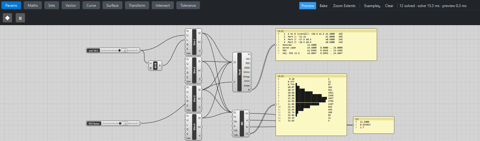
Reference: choose on the canvas toolbar to load the finished definition.
The problem
A gap A–B is set by one overall dimension minus three part dimensions. Following the chain from A to B, the overall dimension points towards B (+) and the three parts point back (−):
| Dimension | Nominal | Tolerance | Direction |
|---|---|---|---|
A to B (overall) |
56.5 |
±1.5 |
+1 |
Part 1 |
11 |
±1 |
−1 |
Part 2 |
17.5 |
±0.5 |
−1 |
Part 3 |
16.5 |
±0.5 |
−1 |
What are the smallest and largest gaps, and how many assemblies fall outside a gap specification of 10 to 13?
Build it
-
Place four Dimension (Tolerance) components, one per row of the table. On each, use Set value… on the inputs:
-
N (nominal), U (upper deviation, for example
1.5) and L (lower deviation, for example-1.5); -
D (direction):
1for the overall dimension,-1for the three parts; -
Nm (name): the label used in the report.
-
-
Place a Stack-up (Tolerance). Wire each Dimension D → Stack-up D, in chain order, holding Shift when you release so the wires are added rather than replaced.
-
Place a Monte Carlo Stack-up (Tolerance). Wire the four Dimensions into its D the same way (with Shift). Set its LSL to
10and USL to13. -
Place three Panels: wire Stack-up R → Panel (the report), Monte Carlo H → Panel (the histogram) and Monte Carlo M, σ and % into a third Panel.
To make the overall tolerance adjustable, add a slider ±tol 56.5: 1.5 (0 – 3), wire it into the first Dimension’s U, and wire it through a Multiplication with B set to -1 into the same Dimension’s L. A second slider RSS factor: 1.5 (1 – 2) wired into Stack-up’s F sets the RSS adjustment factor.
Read the results
The report Panel shows each dimension with its share of the worst-case total, then the three results:
| Method | Tolerance | Gap limits | Meaning |
|---|---|---|---|
Worst case |
±3.5 |
8.0 … 15.0 |
Every tolerance at its limit at once: the gap can never fall outside this. |
RSS |
±1.9365 |
9.5635 … 13.4365 |
√(1.5² + 1² + 0.5² + 0.5²): the probable range if each dimension varies independently. |
Adjusted RSS (× 1.5) |
±2.9047 |
8.5953 … 14.4047 |
RSS with a safety factor for processes that are not perfectly centred. |
Fischer’s book prints ±1.94 and ±2.91 for the last two: he rounds the RSS to 1.94 before multiplying by 1.5. The exact values are the ones above.
The Monte Carlo panel builds 10,000 random assemblies, treating each tolerance as three standard deviations of a normal distribution. Its standard deviation comes out close to RSS / 3 ≈ 0.645, and about 2 % of the builds fall outside 10 – 13. The histogram shows the familiar bell curve.
Things to try
-
Drag ±tol 56.5 down to 0.5. Worst case drops to ±2.5, and the share of rejects falls sharply.
-
Set RSS factor to 1: adjusted RSS equals plain RSS.
-
Set a dimension’s S (distribution) input to
uniformortriangular. Worst case and RSS do not change; the Monte Carlo spread does. -
Change the Monte Carlo Seed to see how much the reject rate moves from one set of 10,000 builds to another.
See Tolerance analysis for the formulas and how each method should be read.